Decision Trees

It is the most simplest Analytics algorithm. It can be used for Regression and Classification purpose.

Regression: We are interested in predicting a continuous variable.

Classification: We are interested in predicting a discrete (Categorical) variable.

Example: A credit card company wants to analyse its previous campaign data to identify potential responders for the upcoming cross-sell offer. Spam or not spam.

We want to send mail to only people who actually reply to the email it credit card is being sold as credit cards are costly.

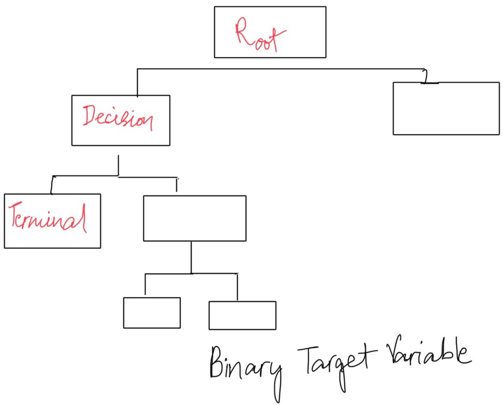
Look at historical data and see who have replied in the past. Root node has all the population present.

In history, 25000 people were sent a mail out of which only 1000 people responded back. Historical rate percent is 1000/25000= 0.4.

We then classify them accordingly to income. 7000 population have high income and there were 460 respondents so the response rate is (460/7000)*100= 6.57 %. If randomly 100 people are picked from population only 6 will respond. There’s an information gain here. The high income is further broken down into age. There is more aged people and less aged people. Out of population of 2000 of more aged there are 360 respondents. The response rate is (360/2000)*100= 18%.

When we spit it further and go deeper, there are more responses.

We future break high age into internet user. Out of population of 100 of high user of internet, 50 respond back, the response rate is 50%.

The decision tree follows a different path. We start with entire population and we keep breaking it on some variable. There is going to be information gain. At each split there’s additional information, that’s the general hypothesis behind this.

How to find out which variable the split should use?

What’s a good split and what’s a bad split. The distribution of root node.

Qualitative way

We assign 1 for target variable and 0 for non-responders.

Quantitative way

These are also called as the purity matrix. They are for categorical target variable.

1. Chi-square
2. Information gain
3. Gini: We need to find what’s the GINI score at the root note. What proportion are the Red Cross and what proportion are the blue cross. Number of Red Cross = 5, Number of Blue cross = 5. Proportion of red= 0.5, Proportion of Blue= 0.5. GINI= (0.5)^2 + (0.5)^2 = 0.5

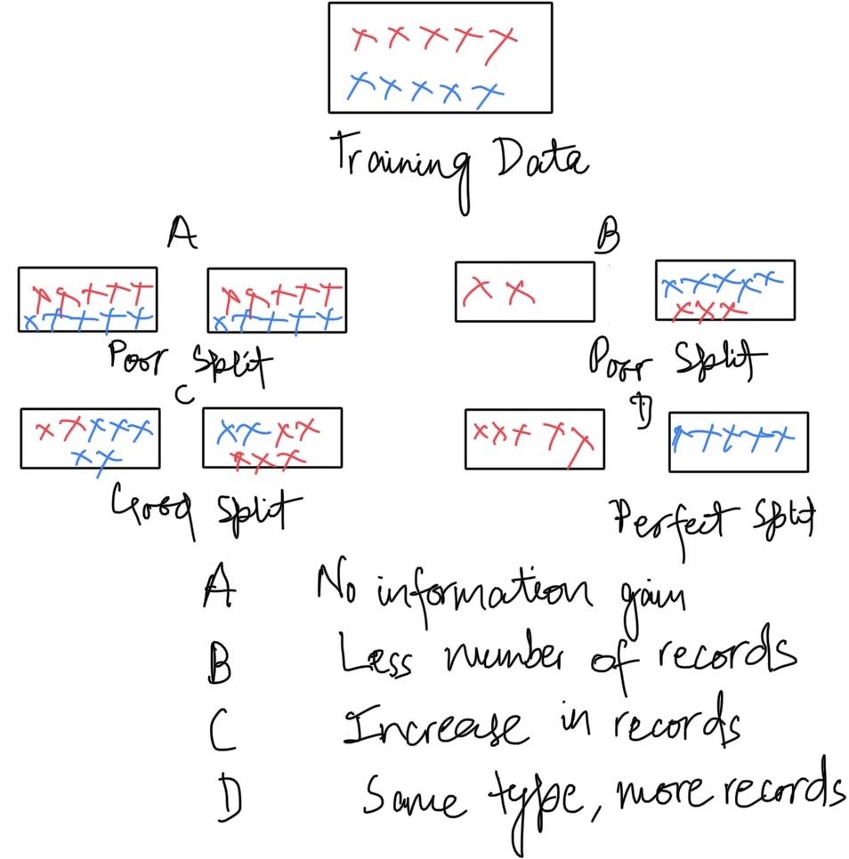
This is the base line of variable. Now we have two variables and we want to find the GINI at the split. The higher the score, the better the split.

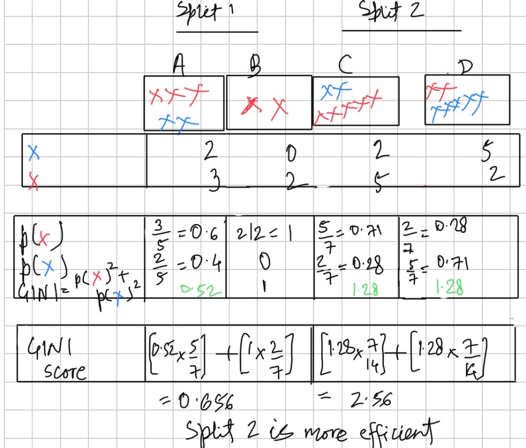
Decision tree penalises if it has lower observation. Split is efficient if it is making high class imbalance. There’s no information gain if the classes are balanced. Higher the class imbalance better the split.

What should be the depth of the tree. It is also called the hyper parameter of the tree. How to decide when the node should be split into two. What’s the stopping criteria of split. Whenever there’s observations less than 100 don’t split.

Decide the hyper parameters to tune:

• How depth should it go.
• What’s the stopping criteria.
• Which purity matrix to use- GINI, Information Gain and Chi-square.

Problem with tree:

Decision trees are prone to overfitting. Overfitting and under fitting both aren’t good.