Decision Trees Case Study

Let ‘dat’ be the dataset name and ‘myt’ be the column name.

Steps involved for decision tree:

1. Import dataset
2. Create dummies out of the categorical dataset
3. Separate featured from the target variable/labels.
4. Then we break it into training labels and testing labels.
5. We call the decision tree algorithm
6. We fit our data into training sets and testing sets.
7. Score the model on testing features and labels.
8. Generate confusion matrix
9. Visualise a decision tree.

dat.isnull().sum() helps find out the missing values.

dat[‘myt’].describe() we want to describe the column types. This gives count, mean, std, min, 25%,50%,75% and max. Let’s assume we get the median as 4.

dat[‘myt’].fillna(4, inplace= True) helps replace the missing values with the median. In place= True, assigns value to the column.

We need to create data frame which contains only input features. We want to drop dependant variable. We want to keep independent variables which are the features.

Y= dat.drop(“default”, axis=1); Axis= 1 means drop should happen on column.

Then convert categorical variables into dummies. Dummies help pass values to the model.

Y= pd.get_dummies(Y)

After that there are full features (independent variables in the column).

X= dat[‘dependant’] We create data frame for dependant variable or target variables.

Next we break our model into training and testing set. The need of this is to test the performance of our model.

import sklearn.model_selection as model_selection

The purpose of random state to make sure the sample is reproducible. It takes values randomly from the dataset.

X_train, X_test, Y_train, Y_test = model.selection.train_test_split(X,Y,test_size= 0.2, random_state= 7)

X_train= target/training labels

X_test= target/training labels

Y_test= Training features

Y_train= Testing features

Suppose Y.shape= 100, 10 (rows, columns)

Y_train.shape= 80,10

Y_test.shape= 20,10

X_test.shape= 20,

X_train.shape= 80,

X_test, Y_test helps check the performance of the model. X_train, Y_train is used to train the model.

We then build tree and import suitable library.

import sklearn.tree as tree

clf = tree.DecisionTreeClassifier(max_depth = 3, random_state= 200)

clf object creates the tree type to fit decision tree. Model fit will happen on training features and labels.

clf.fit(X_train, Y_train)

clf.score(X_test, Y_test) This helps tell the accuracy of the model. Accuracy is how correct is the predicted label of testing set from the actual label in the testing set. To improve accuracy we need to play with hyper parameters like how many levels, what’s the depth etc.

Confusion matrix is the cross tabulation between actual values and the predicted values. It’s the key matrix for all the classifiers.

Import sklearn.metrics as metrics

Metrics.confusion_matrix(X_test, clf.predict(X_test)

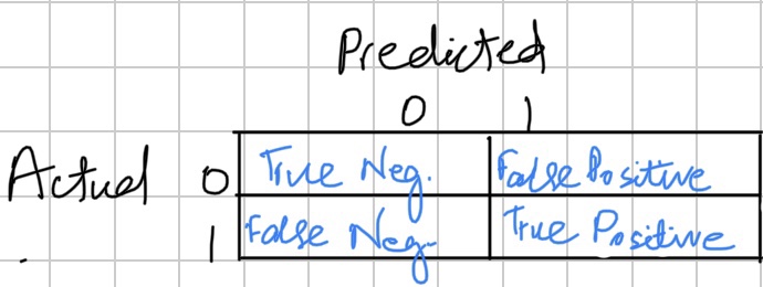
Properly classified:

1. Properly classified: (True negative + True positive)
2. Improperly classified: (False positive + False negative)
3. Accuracy = (True positive + True negative)/ (True positive + True negative + False positive + False negative)

!pip install pydotplus

Import pydotplus

os.environ[“PATH”] += os.pathsep

os.chdir(data_dir)