Make a story out of the data.
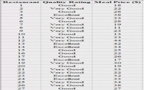
Total restaurant: 300
Sample study: 300, Population size: unknown
Presenter of data: host/
Analyst: Guest/statistics
| Elements/respondents/subjects/Cases |
| 300 |
If restaurant had a name it would be nominal variable.
| Quality Rating | |||
| Categorical variable | Ordinal variable | Nominal variable | Numeric variable /Quantitative/scale variable |
| X1= Good (1) | Male | Meal price | |
| X2= V Good (2) | Female | ||
| X3= excellent (3) |
Meal price is y variable
Quality is x variable
Directionality or relationship between x-y
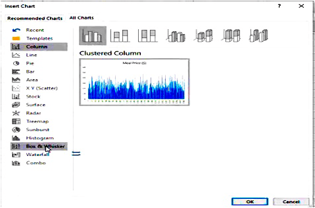
For data analysis in Excel :
Data>Data Analysis
or
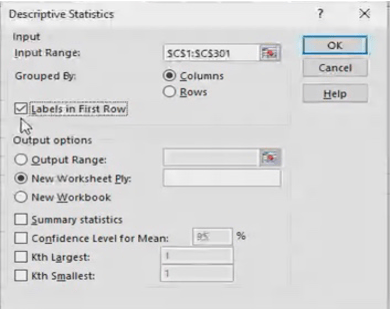
File>options>Excel options>Add-Ins>Analysis ToolPak>Go>OK>check box for Analysis ToolPak
| Function | In excel | ||
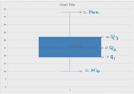
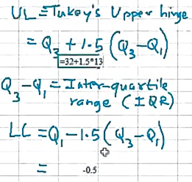
| Mean | =AVERAGE (c2 :c301) | X bar= summ | Quartile : 1/4th of something Q0 : MinimumQ1 : Lower quartile Q2 : Lower quartileQ3 : upper quartileQ4 : maximum |
| Median/Quartile 2 (Q2) | =MEDIAN(c 2 :c301) | Put all in ascending order and find the middle value | Omit largest and smallest value : QUARTILE.EXC |
| Includes largest and smallest : QUARTILE.INC |
| Quartile Num | Quartile | What we did? | Result |
| 0 | =QUARTILE($C$2-$C301) | Freeze array or row (Absolute referencing) | 10 |
| 1 | 19 | ||
| 2 | 25 | ||
| 3 | 32 | ||
| 4 | 48 |
Percentiles (P)
They are the participation values that divide the data into 100 parts.
(n-1) cuts are required to cut into n parts.
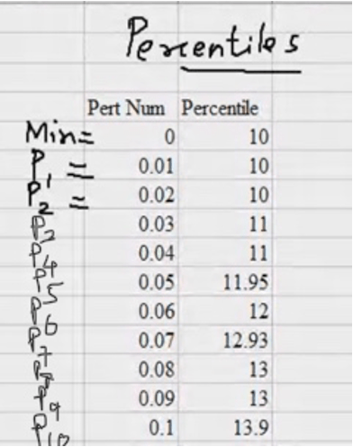
| Percentile number/value | Function | Array | Absolute referencing |
| 0 | =PERCENTILE(Array) | (C2 :C301) | ($C$2 :$C$301) |
| 0.01 | |||
| 0.02 | |||
| 0.03 |
Mode : Most repeated value
Empirical relationship (based on large data) between mean, median and mode.
Help us summarize information in a meaningful way. Help us create a mental picture of data.
“the science that deals with the collection, classification, analysis, and interpretation of numerical facts or data, and that, by use of mathematical theories of probability, imposes order and regularity on aggregates of more or less disparate elements.”
Two parts to the definition:
1. the collection, classification, analysis and interpretation of numeric data
2. the use of probability theory to impose order on aggregates of data
In general, statistics summarizes information about data in a meaningful, relevant way.
Describe the population of Bangalore?
– population in 2010 is 5.4 million
• That is a statistic – the total sum of all full-time residents of Bangalore.
“Population density” “Median Age” “Distribution by Religion” “Literacy Rate”
All these statistics summarize information because talking about each data point is impossible.
Measure of Central Tendency
- Sum: Total of all values in dataset
- Mean: The average of all values in the dataset
- Median: Mid value of sorted data • If even series?
- Mode: Most commonly occurring value in a series
- Minimum: Lowest value in series
- Maximum: Highest value in series
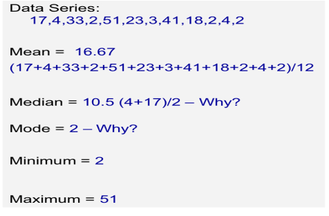
2, 2, 2, 3, 4, 4, 17, 18, 23, 33, 41, 51 : Ascending order of the series.
We can describe the series we looked at in the previous example as: “Minimum of 2, Maximum of 51, Average of 16.6.”
➢ Given this description of the data series, what picture do we form of the data?
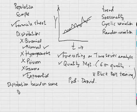
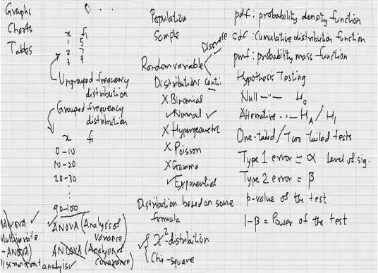
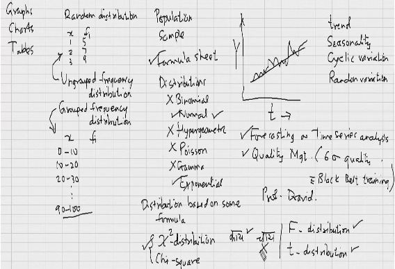
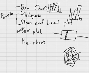
➢ The easiest way to visualize data is to look at its “distribution”
A distribution is a visualization of a frequency distribution table
Taking the data series –
17,4,33,2,51,23,3,41,18,2,4,2
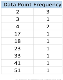
• We create a frequency table which is just counting the number of times each value appears in the data series
• The table shows the frequency count of each data value
• A better way to create this table would be to use ranges of values, rather than individual data points.
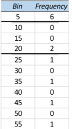
Bin refers to the value range, so 5 refers to “0 – 5”
• We have 6 observations that have values between 0 – 5,
2 observations with values between 15 – 20 and so on
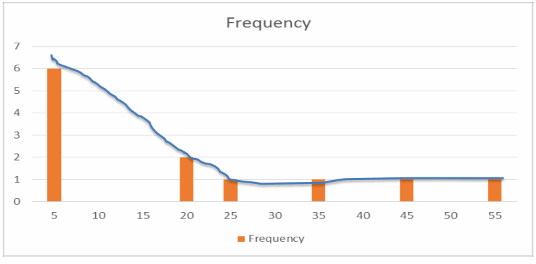
• The quickest way make sense of this data is to turn it into a visualization.
Measure of dispersion
For Example:
- Range
- Variance
- Standard Deviation
Application and use of standard deviation :
Chebyshev’s inequality
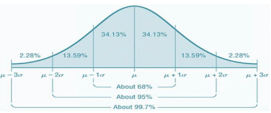
For any data set, it can be proved mathematically that –
- Atleast 75% of all data points will lie within 2 std deviations of the mean, ▪ atleast 89% of all data points will lie within 3 std deviations of the mean.
- For a data series with a min of 200, max of 1500, a mean of 600, and a std deviation of 80,
- Atleast 75% of all the data points in the series will be within the range: 600 – 2*80, 600 + 2*80 : (440, 760)
- Atleast 89% of all data points in the series will be within the range: 600 – 3*80, 600 + 3*80 : (360, 840)
Example: Standard deviation as a sense of variation in data.
Supposing we had data on customer spend by store.
Average spend per customer in Store Awas $150, with a std deviation of $35, and the average spend per customer in Store B was $145, with a std deviation of $15.
In which store are sales higher?
Example: Standard deviation used as a measure of risk.
You are trying to pick stock for investing in the equity market.
- ▪Stock A has an annual return of15%, with a std deviation of 30%
- Stock B has an annual return of 12%, with a std deviation of 8%
- If you were risk averse, which would you choose?
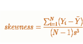
Measures of Shape
- The degree of skewness
- Skewness is the absence of symmetry
- A symmetric shape is one where the left side of the data distribution is a mirror image of the right (side relative to mean)
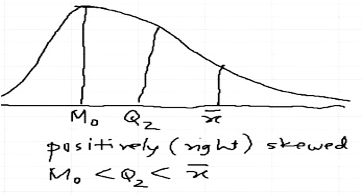
- Positive Skew: Long tail to the Right
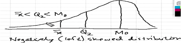
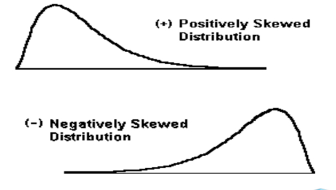
- Negative Skew: Long tail to the Left
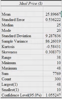
Distribution of meal prices approximately symmetric :
The distribution of meal price is slightly positively symmetric:
The distribution of meal price is slightly negatively symmetric: If below -2 in number line
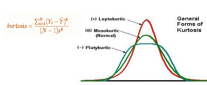
- Kurtosis: Sharpness of the peak of the distribution. Co-efficient of Kurtosis is an index/value of peakeeness/tallness of the data.
- A high kurtosis distribution has a sharp peak and fat tails
A low kurtosis distribution has a flat peak and thin tails
Leptokurtic: The kurtosis is greater than 0.
Mesokurtic : coefficient of Kurtosis is equal to 0.
Platykurtic: The coefficient of Kurtosis is less than 0.
Why is it important to learn about summary statistics?
- Description of a large number of data points
- Generate inference from the summary statistics
Example:
You work for a credit card company and are required to understand drivers of default.
You have access to :
- Billing data
- Demographic data
You divide the data into customers who have:
1. A great payment record, and
2. Customers who have been late with payments at least 3 times in the last year
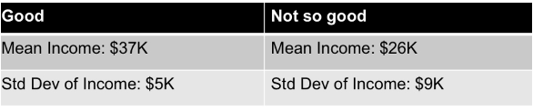
Mean income – capacity to pay back
Lower income is not so good, but higher income is Good
Standard Deviation – larger the std deviation, greater the variation in income
Variation in income is higher in Not so good, implying there is an overlap in income in Good and Not so good.
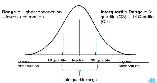
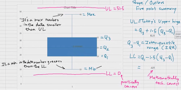
Q3 : 75% observations have less value than x.
Q2 : 50% observations have less value than x2.
Q1 : 25% observations have less than x1.
Rating is ordinal as we can order.
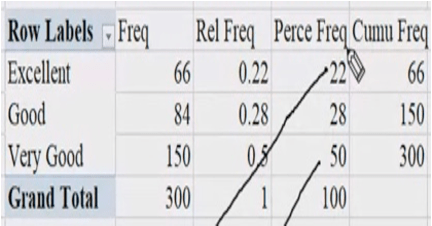
Rank 1 : Excellent
Rank 2 : v. Good
Rank 3 : Good
Rank 4 : Satisfactory
Rank 5 : unsatisfactory
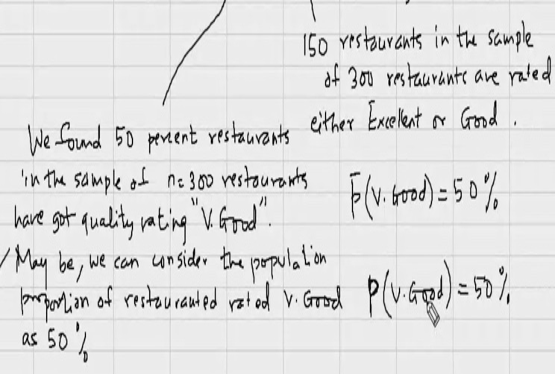
150 restaurants in the sample of 300 restaurants are rated either excellent or good.
Normal probability distribution
It is a continuous probability distribution.
What is a discrete distribution?
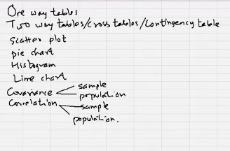
One way frequency table
| Xi | Fi | Relative frequency |
Two way frequency table
| X/y | Y1 | Y2 |
| X1 | ||
| X2 |
Joint probability table represents joint distribution of two variables.
The important requirements of a discrete relative variable is
0<= p(x=xi) <= 1
Summation (n, i=1) P(x= i)=1
Using table or histogram : we cannot use for continuous variables.
The distribution of a Continuous random variable can be represented using a continuous curve or a formula.
Random variables
| Discrete random variables | Continuous random variables |
| Finite : Number it success in n trials. X= 0,1,2,3,…,n | X=Time of arrival between two customers of a shop or mall in minutes [0, infinite]. It assumes or takes values on the interval on a number line. |
| Countable infinite : number of customers visiting a shopping mall, in an hour.X=0,1,2,3 | Area under the curve (Cumulative distribution function) :F(x)= integration p(x<= xi) |
| Volume, size, rainfall, height, weight, time variables change continuously. |
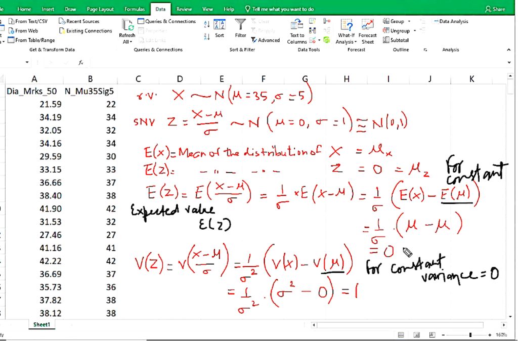
Normal probability distribution
A continuous random variable x~
~ Tild symbol, it means follows Normal (mu, sigma square) if its probability density function (PDF)
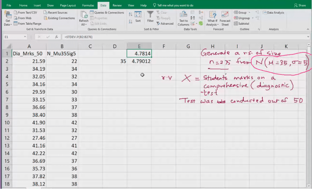
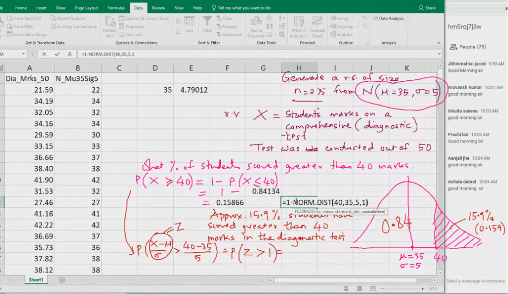
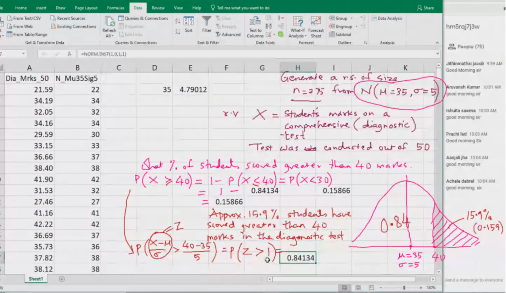
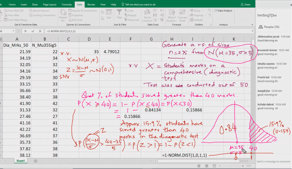
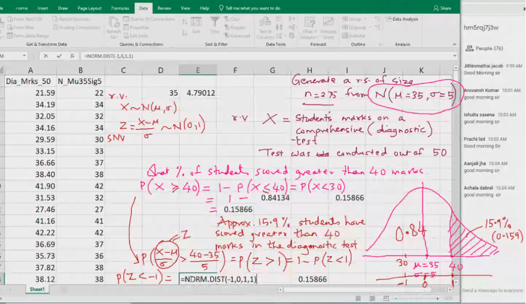
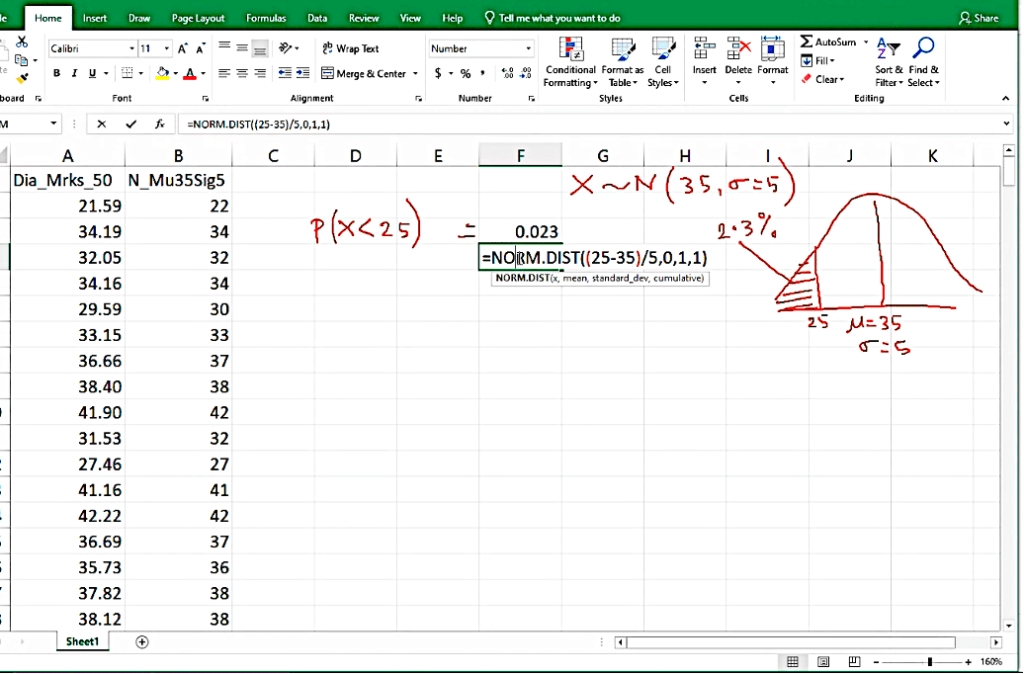
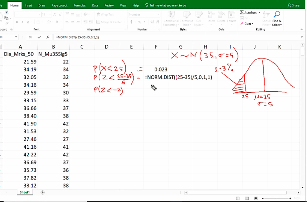
When we want to calculate area we put probability distribution fucntion.
Z-score: Standard deviation 30 is below 35
Sampling
N=5, n=2
No of possible outcome= = 10=
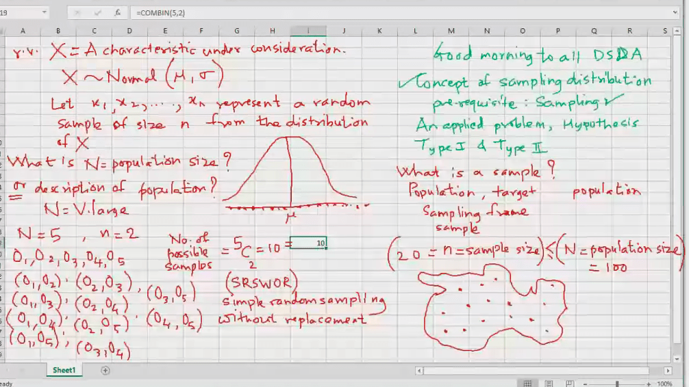
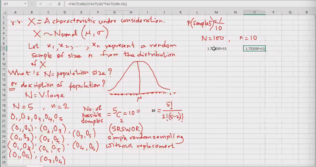
When the population sample is 100 and sample is 10 there are alot of random samples.
We need the sampling distribution of sample statistics here
x
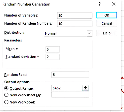
Let the number of random samples= 80
Size of each sample= 10
Data>Data Analysis > Random Number Generation
