listwise deletion method?
It ignores complete row where there is missing value
Why CRISP-DM?
- The data mining process must be reliable and repeatable by people with little data mining skills
- CRISP-DM provides a uniform framework for :
- Guidelines
- Experiential documentation
- CRISP-DM is flexible to account for differences
- Different business/agency problems
- Different data
1. Business Understanding: This initial phase focused on understanding the project objectives and requirements from the business perspective and then converting this knowledge into a data mining problem definition, and a preliminary plan designed to achieve the objectives.
2. Data Understanding: The data understanding phase starts with an initial data collection and proceeds with activities in order to get familiar with the data, to identify data quality problems, to discover first insights into the data, or to detect interesting subsets to form hypotheses for hidden information.
3. Data Preparation: The data preparation phase covers all activities to construct the final dataset (data that will be fed into the modelling tool(s)) from the initial raw data. Data preparation tasks are likely to be performed multiple times, and not in any prescribed order. Tasks include table, record, and attribute selection as well as transformation and cleaning of data for modelling tools.
4. Modelling: In this phase, various modelling techniques are selected and applied, and their parameters are calibrated to optimal values. Typically, there are several techniques for the same data mining problem type. Some techniques have specific requirements on the form of data. Therefore, stepping back to the data preparation phase is often needed.
5. Evaluation: At this stage in the project you have built a model (or models) that appears to have high quality, from a data analysis perspective. Before proceeding to final deployment of the model, it is important to more thoroughly evaluate the model, and review the steps executed to construct the model, to be certain it properly achieves the business objectives. A key objective is to determine if there is some important business issue that has not been sufficiently considered. At the end of this phase, a decision on the use of the data mining results should be reached.
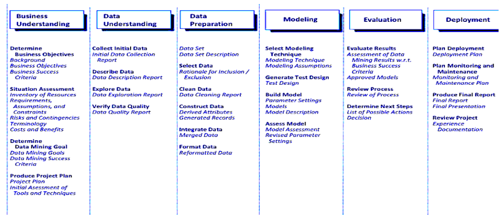
6. Deployment: The creation of the model is generally not the end of the project. Even if the purpose of the model is to increase knowledge of the data, the knowledge gained will need to be organized and presented in a way that the customer can use it. Depending on the requirements, the deployment phase can be as simple as generating a report or as complex as implementing a repeatable data mining process. In many cases, it will be the customer, not the data analyst, who will carry out the deployment steps. However, even if the analyst will not carry out the deployment effort it is important for the customer to understand upfront what actions will need to be carried out in order to actually make use of the created models
Data Quality: Why pre-process the Data?
Pandas is used for storing data in a tabular form.
read_CSV
Shape
Info ()
The types
Kollam
Crosstab
Pivot_table
Drop: delete Rows and columns
Rename: change name of the column.
https://www.saedsayad.com/oner.htm
str(weatherdata)
model<-
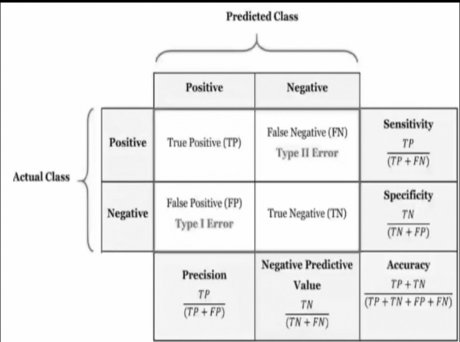
Rows: Actual values
Columns: Predicted values
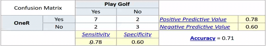
Sensitivity tells whether one is able to capture all the true positives or not. Specificity tell us whether one was able to capture all the true negative or not. It’s a risky call if a person has cancer and the model shows false negative, predicting he won’t get cancer even though he is highly likely of getting cancer. In such cases to increase the specificity all the type 2 errors need to be reduced. The metrics are: Accuracy, Precision, Recall, Specificity and F1
True positive : actual is true, correctly predicted : 7
False negative: 2: actual is yes predicted is no.
False positive: actual is no, classifier predicts as true: 2
True negative: actual no predicted no: 3
Person is infected but test says yes false positive
Infected but pcr says negative False negative
Positive
Accuracy: TP+TN/total number of cases (TP+TN+FP+FN)
In reality he is a defaulter but it doesn’t show that he is one.
compdata<-read.csv(“c:/DS & DA Symbi/buyscomputer.csv”, colClasses =“factor”)
head(compdata)
formula<-buyscomputer~age+income+student+creditrating
j48model<-J48(formula,compdata)
summary(j48model)
install.packages (“partykit”)
Library(partykit)
Plot(j48model)
The independent attributes are used to make dependent attributes. The attribute which provides the best split is used.
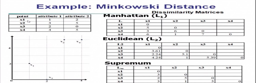
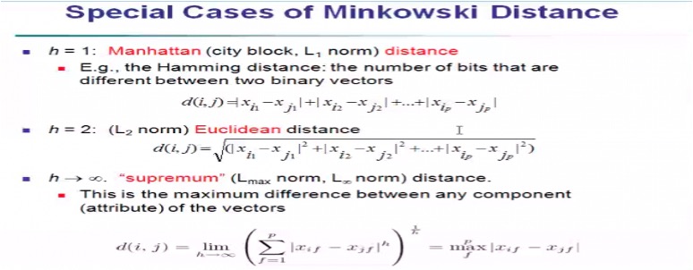
ED= SQRT(X2-X1)^2
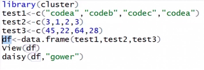
Growers distance formula
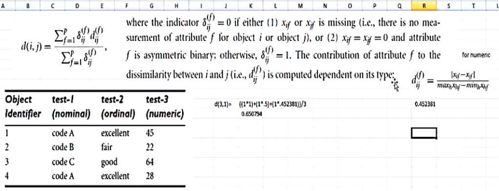
R code for Growers distance.
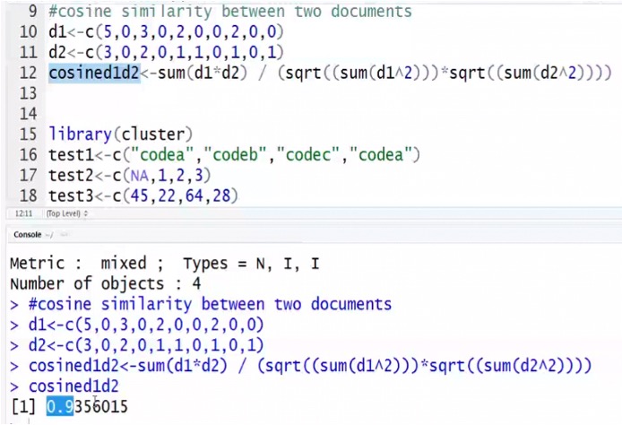
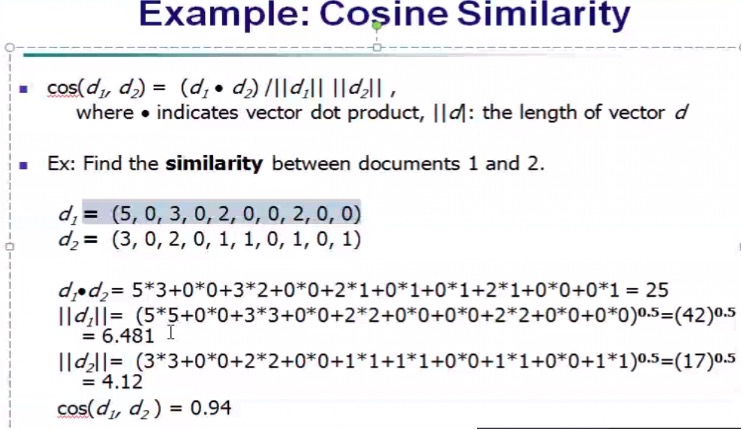
Cosine similarity measure is more suitable to find similarity between two documents?
Implementation of decision tree using R
set.seed(100)
i<-sample(1:nrow(BankSol),.7*nrow(BankSol)) #70% train data
train<- BankSol[i,]
test<- BankSol[-i,]
dim(train)
dim(test)
j48BankSol <-J48(IsDefaulted~.,train)
summary(j48BankSol)
testpred <- predict(j48BankSol,newdata=test)
table(test$IsDefaulted,testpred)
(sum(testpred==test$IsDefaulted)/nrow(test))*100
iris
i<-sample(1:nrow(iris),.7*nrow(iris))
train <- iris[i,]
test<- iris[-i,]
dim(train)
dim(test)
j48BankSol <-J48(Species~.,train)
summary(j48BankSol)
testpred <- predict(j48BankSol,newdata=test)
table(test$Species,testpred)
(sum(testpred==test$IsDefaulted)/nrow(test))*100
| a | b |
| 353 | 4 |
| 34 | 98 |
a=0, b=1
(34+98) = 134 total positive
Tota negative : 357
1 defaulter
0 is non defaulter
98 are defaulter, correctly predicted : True positive
353 are non-defaulter and identified as non-defaulter : true negative
34: Defaulters but model is predicting them as non-defaulters : False negative
4 are non-defaulters but model is predicting them as defaulters : False positive
| 0 | 1 | |
| 0 | 137 | 23 |
| 1 | 33 | 18 |
True negative : 137
False positive : 23
False negative : 33
True positive : 18
(137+18) /211 : 73.45% predicted.
The model is 73.45% accurate.
Model is not able to predict the unseen data properly (test data accuracy)
How accurately the data is able to predict the seen data (training data accuracy)
Training accuracy is better than the test accuracy.
Overfitting : when it is not to generalise. It can predict what it has seen and not unseen.
Training 60% test 55%. It’s not even good on seen and unseen data. Anything below is 50%. Underfit data.
Above 75% accuracy is good.
Overfit :
90% training
70% test data
| setosa | versicolor | virginica | |
| Setosa | 11 | 0 | 0 |
| versicolor | 0 | 14 | 0 |
| virginica | 0 | 3 | 17 |
Test : 93%
Training : 98%
(11+14+17)/(11+14+17+3)=
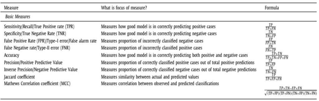
F1 score = (2*precision*recall)/(precision+recall)
Attribute selection:
- Entropy
- Gain ratio
- Gini index: It strictly generates binary tree. Gender is symmetric binary a!ribute
Which algorithm creates strict binary tree and which creates non-binary tree.
How many negative cases are predicted correctly as negative: sensitivity
What is positively predicted value:
Precision. It is used on the data status imbalanced.
= TP/(TP+FP)
It is positive but incorrect.
correctly classifying maximum number of positive cases without compromising much on incorrect prediction of negative case or positive predictive value: Precision.
True positive: how many are correctly predicted as positive.
True negative: how many negative cases are correctly predicted as negative
False positive: how many negative cases incorrectly predicted as positive
False negative: How many positive cases are incorrectly predicted as negative
Total positive: (FN+TP).
Total negative: (TN+ FP)
Sensitivity: out of total actual positive cases how many are correctly predicted as positive equal to tP/P.
= TP/(TP+FN)
Specificity: out of total active negative cases how many or correctly predicted as negative.
= TN/N
= TN/ (TN+FP)
Precision: out of total positive predictions how many or actually positive
=TP/(TP+ FP)
Inverse precision: out of total negative precision how many are actually negative.
= TN/(TN+ FN)
Accuracy: (TP
Out of total cases how many are correctly predicted as positive and negative.
It doesn’t measure reflect the true performance of the classifier if your dataset is highly imbalanced.
Popular ensemble models:
- Bagging: averaging the prediction over a collection of classifiers.
- Boosting: weighted vote with a collection of classifiers.
- Ensemble: Combining set of heterogeneous classifiers. Different classifiers can be built through support vector, artificial neural networks, naïve Bayes, random forest.
Ensemble methods:
Uses a combination of models to increase the accuracy of the classifier.
Combine a series of methods
In case of prediction problem, find mean of all.
For categorical for with majority of votes.
Random forest:
In the decision tree classifier, there’s only one thing in running Forrester of several trees using different samples and then the results are combined of all the classifiers and that result will be the final decision. In random forests instead of building a single decision tree, several decision trees are felled and the results are combined. In bagging several samples or created a classified as created the classify could be a knife-based classifier or a random forest classify. In the case of a random forest when
Bagging and random forest: all attributes are potential for selection
In a random forest, it randomly selects randomly for reducing the risk.
Ada-boost: a famous algorithm for building and classifying a model.
Imbalanced: the performance won’t be that great.
Oversampling:
Under-sampling: reduce the majority of cases.
Hybrid methods:
Refer research paper got balanced and imbalanced datasets.
Best predictions
J48 classifiers, homogeneous ensemble method is bagging.
What’s the difference between random forest and bagging?
Both are homogenous.
What are the problems with homogeneous ensemble methods?
Random forest considers the square root of n features so each time the sample is different.
Under-root of features for the random forest.
All features are considered for splitting in the decision tree.
GINI index tells about the best attributes.
What’s the stopping criteria for the k-mean criteria?
It is sensitive to outliers.
