Data structure:
- Vector
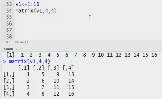
- Matrix
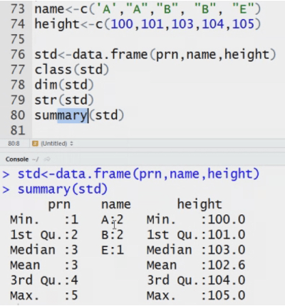
- Data frame
- List
R is a case sensitive language.
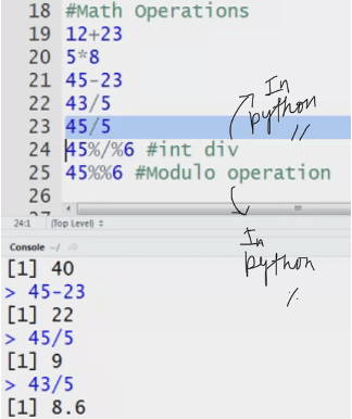
Addition in R:
A+b
No need to declare the variable in R and Python.
In python type to check the Datatype of variable.
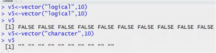
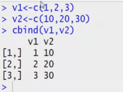
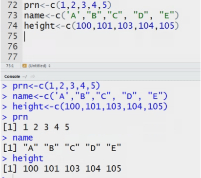
How to create vector in R?
Vector is a 1D array.
Height <- c(165,167,168,160,158)
Function c helps create array from a list.
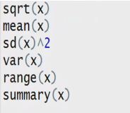
- Sum(): sum of all elements
- Mean(): mean
- Class(): datatype
- Min(): minimum value
- Max(): max value
- Sd(): standard deviation
- Var(): variance
Names<-c(‘a’) data type = character
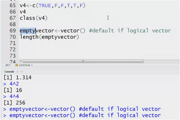
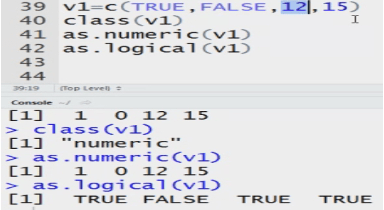
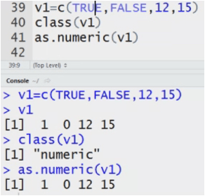
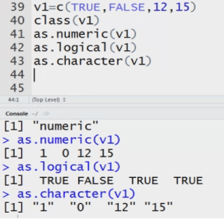
Graduate <- c(TRUE, FALSE, TRUE)
Class(Graduate)
The data type= logical
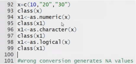
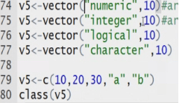
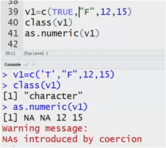
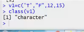
my data<-c(2,3,’a’,’b’) System converts the Datatype to numeric to character.
System can convert numeric into string but not vice versa.
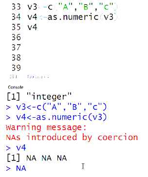
Mydata2<-c(“1”,”2”,”3”)
Class(mydata2)
For explicit conversion from character to numeric.
Mydata3<-as.numeric(mydata2)
Class(mydata3)
Integer and float are both numeric data types.
V1<-(23,45,67.78,65.56,34.56)
Missing value in python: NaN
Missing value in R: Na
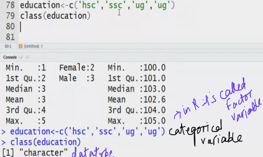
Name can’t be a categorical variable.
Address can be character or string and it has no pre-defines value.
Name can be character or string.
List can store elements of any type:
- Matrix
- Vector
- Data frame
- Numeric
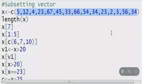
Vectors are mutable. The value of the vectors can be changed. It is used majority of the times.
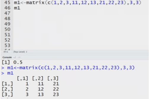
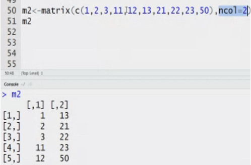
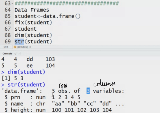
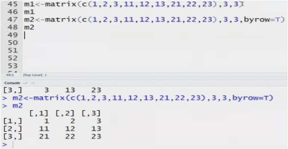
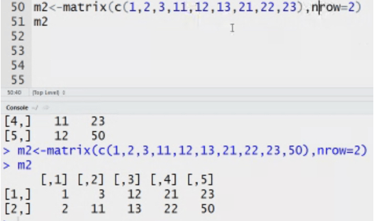
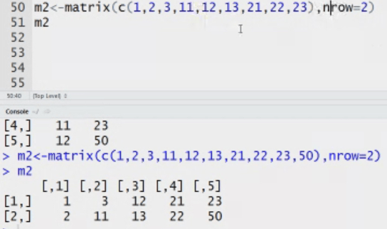
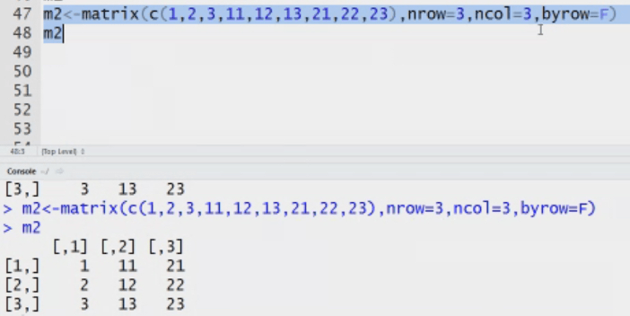
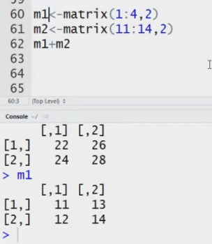
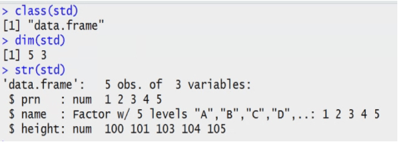
Matrix: n dimensional matrix. The elements of same type. Length of each column is same. It stores value in tabular form.
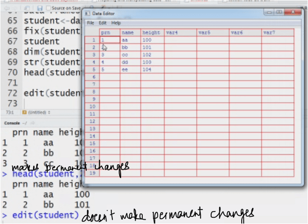
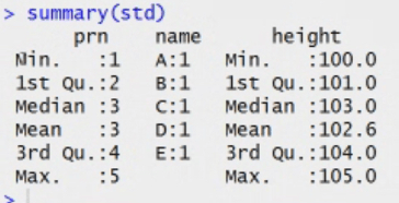
Data frame: how is it different from matrix. It stores data in tabular. It can have different data types.
List: When we want to store any kind of data. It is rarely used. But it is very powerful. It’s multi-dimensional. There can be list within a list.
Hierarchical data type format.
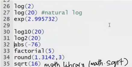
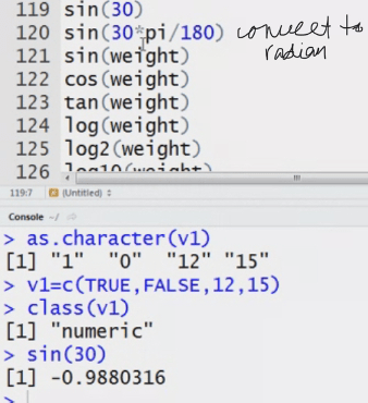
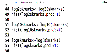
log2(x), log10(x)
Data transformation:
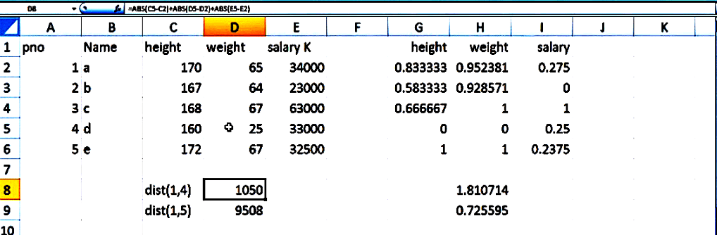
- Min and maximum
- Z score standard scalar
- Decimal scaling= x/10^3 number of digits of maximum values
- Log transformation
- Sqrt transformation
- Discretisation
height<-c(170,167,168,160,172)
zvalue=(height-mean(height))/sd(height)
zvalue
height<-c(170,167,168,160,172)
dscaling=height/10^3
height=(height-min(height))/(max(height)-min(height))
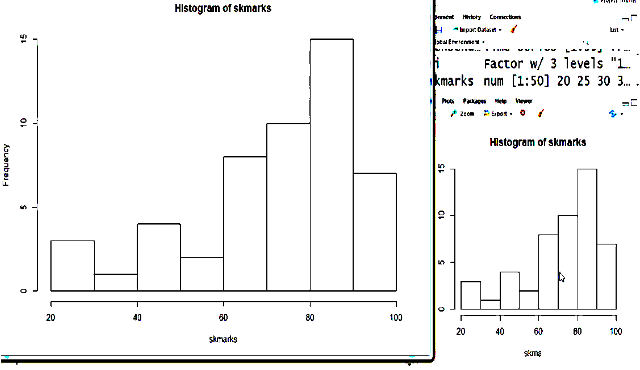
It is left skewed normal distribution. It’s negatively skewed.
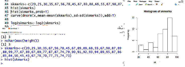
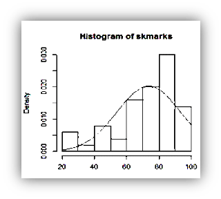
curve(dnorm(x,mean=mean(skmarks),sd=sd(skmarks)),add=T) adds the curve to the graph.
add=T adds the curve
To make the distribution normal
Negatively skewed is not applicable for log transformation, square root transformation according to a research.
Left skewed transformation/Negatively skewed is applicable for square transformation and cube transformation according to a research.
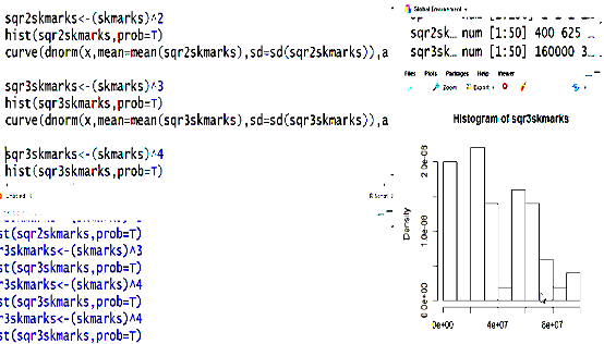
Log and sqrt transformation for negatively skewed distribution and we want to transform it to normal distribution.
gender<-c(“male”,”female”,”male”,”female”,”male”, “male”)
table(gender)
We want to convert categorical data to numeric form.
gender[gender==’male’]=1
gender[gender==’female’]=2
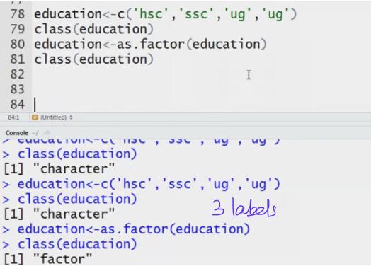
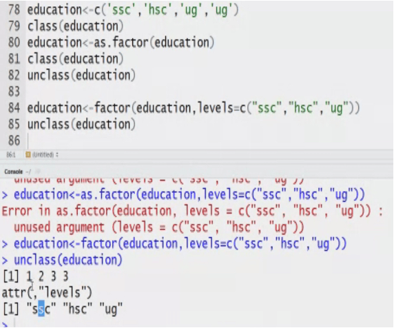
gender=as.factor(gender)
Read.csv(name of file, sep=“;”)
Read.tavle(name of file, sep=“\t”, header= T)
SomeData<-read.csv(name of file,Sep=“,”, header=F, col.names=c(“Name”,”City”),na.strings=c(“”,”,”,” “)
SomeData<- read.csv(name of file,Sep=“,”, header=F, col.names=c(“Name”,”City”),na.strings=c(“”,”,”,” “), slip=3, comment.char=“$”)
- Unstructured data : voice, audio
- Structured data : Data in a tabular form. Regional database, SQL, etc.
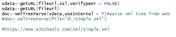
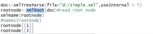
- Semi structured : XML, Jason, No structure
XML package:
Mean is always sensitive to the outliers, it changes due to the outliers.
mean <- ifelse(is.na(airquality$Ozone)
mean(airquality$Ozone, na.rm=TRUE)
airquality$Ozone)
airdata<-airquality
for(i in 1: ncol(airdata))
{
airdata(is.na(airdata[,i}),i]<-mean(airdata[,i],na.rm = TRUE)
}
airdata
https://www.tandfonline.com/doi/abs/10.1080/08839514.2019.1637138
